The Grid Was Never Built for This

The chatbot that wrote all your AI slop last week learned everything it knows inside a four-line for loop. Run that loop on 100k GPUs, and one line can shake the grid hard enough that regulators have started regulating data centers like power plants.

The Training Loop

A neural network is a function with billions of tunable parameters, and training is the process of nudging each one in the direction that makes the AI model’s predictions less wrong. Every parameter gets its own number answering one question: If we nudge this parameter up a little, does the model’s mistake get bigger or smaller, and by how much? That number is the gradient.

Real training uses a mechanism called autograd to get every gradient at once. PyTorch’s loss.backward() traces the arithmetic that produced the loss in reverse and deposits a gradient on every parameter in one call. With gradients in hand, training is essentially a four-line loop:

for step in range(num_steps):
    logits = model(tokens)           # predict the next token
    loss   = cross_entropy(logits)   # how surprised were we?
    loss.backward()                  # gradients for every parameter
    optimizer.step()                 # nudge each parameter downhill

See the appendix for the bookkeeping behind loss.backward().

Here, the first line runs the input through the model to make predictions. The loss measures how poorly the model predicted the next token. loss.backward() uses the chain rule to work out which direction each parameter should move and how far. Finally, the optimizer nudges all the parameters accordingly.

100k GPUs

A frontier model trains on trillions of tokens, far more than one GPU can process in any useful amount of time. At that scale, we need 100k GPUs working through the pile at once. In the simplest version, every GPU holds a copy of the model and sees a different slice of the data. Each one runs the same training loop and computes its own gradients, and then the fleet combines the results. This is called data parallelism.

But those copies come with a fragile invariant. They have to stay identical. If one of the GPUs updates its parameters using only what it learned from its own slice of data, it now holds a slightly different model from everyone else’s. Within a few hundred steps, we’re no longer training one model. We end up training 100k models that have drifted apart. So we add one more step to our loop:

    loss.backward()             # every parameter now holds its .grad
+   all_reduce(model.grads)     # average gradients across every GPU
    optimizer.step()

all_reduce(model.grads) is a collective operation where each GPU sends out the gradients it learned from its own slice of data. The cluster averages them and sends the shared result back to the GPUs so that every copy of the model stays in sync. The problem is that the average cannot be calculated until every GPU has finished computing its gradients, so the fastest GPUs must wait for the slowest. In each iteration, the averaging step becomes a synchronization barrier, holding the entire cluster until every GPU has the same gradients. Only then can the GPUs update their copies of the model, and a months-long training run hits that barrier millions of times.

The Waveform

Each loop iteration has two electrical modes. While a GPU is computing predictions and gradients, its tensor cores are saturated and the chip runs near full power. During all_reduce, the chip shares gradients over the network and sits idle until the average comes back. Power usage falls by hundreds of watts.

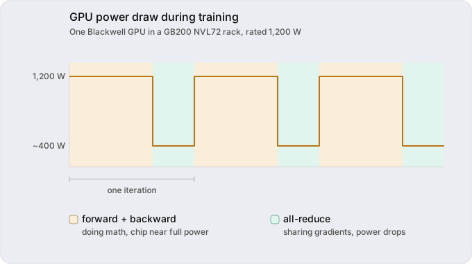
Power also fluctuates when millions of users talk to a chatbot, but their requests arrive at random moments, so most of those fluctuations cancel each other out. A training run does not have the same randomness. In each iteration, all_reduce(model.grads) takes any GPU that has drifted ahead and holds it until the rest arrive. This forced alignment is not an accident or a bug to engineer away; it is produced, deliberately and continuously, by the definition of the training job. The GPUs ramp up in power consumption and taper off together, so the waves do not cancel. They stack into a power draw that pulses every second or so, locked to the rhythm of the training loop. While the size of the swings is manageable, the speed is a threat because the pattern runs up against how power plants are designed to work.

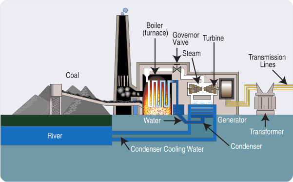
A power plant does not answer a change in demand all at once. It responds in layers:

• When demand rises somewhere on the grid, the generator feels it within milliseconds. More current flows through its windings, and that current sets up a magnetic field that drags against the spinning rotor.
• The heavy shaft between the turbine and the generator slows as the generator draws on the rotating machinery’s stored energy and supplies the grid.
• The governor notices the lost speed and opens the steam valve. More steam pushes on the turbine blades, adding energy until the plant is back in balance with the grid.
• Grid controls and operators draw on reserves by ramping other generators, discharging batteries, or importing power from neighboring grids to balance the new load across the system.

A training run’s power draw creates a square wave. It swings hundreds of megawatts in lockstep, up and down about every second. That rhythm is too quick for a power plant’s governor to fully smooth out and too sudden for an operator watching the grid to correct manually. When the load rises, the current through the generator changes almost immediately. The turbine, which has to wait for valves and steam flow, responds slowly. If the load stepped up once, the plant would absorb it as a normal bump in frequency. But the training run never gives it a chance to settle, raising and dropping the load again and again, and the shaft between the turbine and generator twists back and forth with every iteration of the training loop.

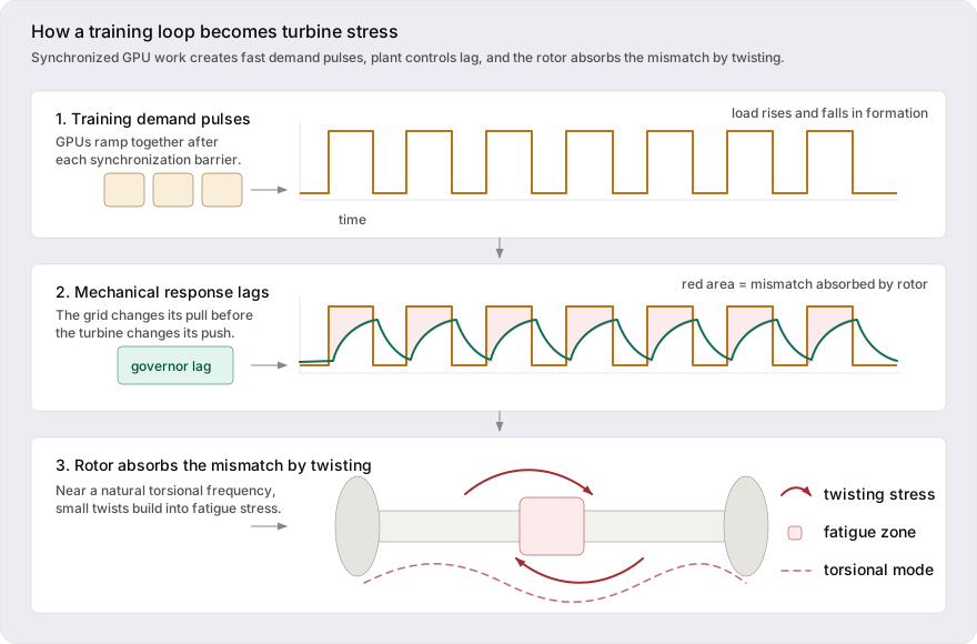
The twist itself is not the danger, but the repetition is. Turbine shafts are built to hold enormous steady loads, but repeated twisting can cause metal to fatigue. If the pulses arrive at the wrong rhythm, near one of the shaft’s natural torsional frequencies, each twist can reinforce the last. Over time, that repeated stress can turn an electrical waveform into fatigue in steel. Each cycle adds a little more strain, until the shaft cracks.

Shipping the Fix

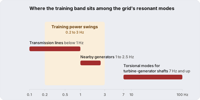
In August 2025, Microsoft, OpenAI, and Nvidia published a joint paper, "Power Stabilization for AI Training Datacenters", based on measurements from production training clusters. The paper found that synchronized training could move a single data center’s power demand by tens of megawatts, and potentially hundreds when a job spans enough machines. The frequency of the swings was as important as their magnitude. In real training traces, much of the waveform’s energy clustered between 0.2 and 3 Hz, the same band where long transmission lines and neighboring generators naturally oscillate, and a repeated load arriving inside that band can amplify those oscillations instead of letting them die out. Turbine-generator shafts have their own danger zone higher up, beginning around 7 Hz.

Nvidia GPUs now ship a power-smoothing feature that deliberately burns extra energy to make training loads easier for the grid to absorb. It holds GPUs above a minimum power floor and limits how quickly their power draw can rise or fall, rounding off the square wave before it reaches the utility. In the paper’s tests, the floor kept every GPU above 90 percent of its rated power, even while the chip sat waiting on all_reduce, and that idle draw added about 10.5 percent to the energy bill of the training run.

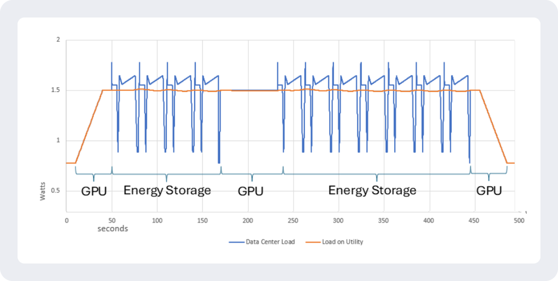
Finally, regulators stepped in. NERC, the body that polices grid reliability, spent 2025 escalating from reports to alerts about load swings too fast for operators to correct. In July 2026, FERC ordered NERC to write mandatory reliability standards for what it now calls computational loads, pulling data centers into the same rulebook as power plants. For twenty years we kept the grid stable by regulating supply. Now we also have to regulate demand.

Appendix: Autograd from Scratch

We could get gradients by brute force. Nudge one parameter, run the input through the entire model again, and measure what changed. For a model with billions of parameters, that would mean rerunning it billions of times just to take one training step. Autograd gets the same answer without trying every parameter one by one.

Here is what a parameter value looks like in Python:

class Value:
    def __init__(self, data, children=(), local_grads=()):
        self.data = data              # the number
        self.grad = 0                 # d(loss)/d(this), filled in later
        self._children = children     # what produced this value
        self._local_grads = local_grads

    def __mul__(self, other):
        # d(a*b)/da = b, and d(a*b)/db = a
        return Value(self.data * other.data, (self, other),
                     (other.data, self.data))

    def __add__(self, other):
        return Value(self.data + other.data, (self, other), (1, 1))

    def backward(self):
        self.grad = 1  # d(loss)/d(loss) = 1
        for v in reversed(topological_order(self)):
            for child, local in zip(v._children, v._local_grads):
                child.grad += local * v.grad   # chain rule

Every multiply and add returns a new Value that remembers its inputs and the local derivative of the operation. Stack enough of these operations together, and their links form a computation graph. When we call .backward() on the final result, the chain rule walks that graph in reverse, depositing a gradient on every node it passes.

a = Value(2.0)
b = Value(3.0)
loss = a * b + a      # loss = 8.0
loss.backward()
a.grad                # 4.0. nudge a up by 0.001, loss rises by ~0.004
b.grad                # 2.0

PyTorch’s loss.backward() does the same reverse walk over tensors instead of single numbers. Modern AI chips do the underlying multiply-adds by the trillions.